
Understanding Generative Adversarial Networks - Part II
In "Understanding Generative Adversarial Networks - Part I" you gained a conceptual understanding of how GAN works. In this post let us get a mathematical understanding of GANs.
The loss functions can be designed most easily using the idea of zero-sum games.
The sum of the costs of all players is 0.
The sum of the costs of all players is 0.
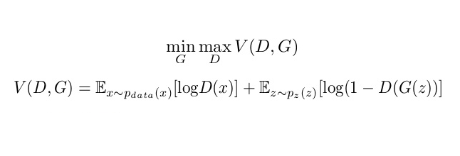
This is the Minimax algorithm for GANs
Let’s break it down.
Some terminology:
V(D, G) : The value function for a minimax game
E(X) : Expectation of a random variable X, also equal to its average value
D(x) : The discriminator output for an input x from real data, represents probability
G(z): The generator's output when its given z from the noise distribution
D(G(z)): Combining the above, this represents the output of the discriminator when
given a generated image G(z) as input
given a generated image G(z) as input
Now, as explained above, the discriminator is the maximizer and hence it tries to
maximize V(D, G). The discriminator wants to correctly label an image from the input
data as real.
maximize V(D, G). The discriminator wants to correctly label an image from the input
data as real.
Thus, it tries to maximize D(x). At the same time, a generated image (created by the
generator), must have a very low chance of coming from the input data -- it should be
fake. Thus, D(G(z)) should be small, or 1 - D(G(z))should be large. And as log is an
increasing function ( it increases with increasing x), one can easily see how V(D, G)
is getting maximized here.
generator), must have a very low chance of coming from the input data -- it should be
fake. Thus, D(G(z)) should be small, or 1 - D(G(z))should be large. And as log is an
increasing function ( it increases with increasing x), one can easily see how V(D, G)
is getting maximized here.
The converse is true for the generator. It wants to increase the chance of the
discriminator incorrectly classifying a generated image as real. Thus, D(G(z)) should be
large. As this term increases, log(1 - D(G(z))decreases. Thus, V(D, G) decreases here.
discriminator incorrectly classifying a generated image as real. Thus, D(G(z)) should be
large. As this term increases, log(1 - D(G(z))decreases. Thus, V(D, G) decreases here.
Now, as we have understood the intuition behind the minimax algorithm for
adversarial networks, let’s discuss the gradients.
adversarial networks, let’s discuss the gradients.

As explained above, the discriminator has to maximize the minimax value function
V(D, G). Thus, it must undergo what is called gradient ascent (yeah.. not descent).
It’s weights must be updated with the above gradient.
Coming to the generator, it must undergo gradient descent with respect to the this:

Now comes the actual implementation:
A for loop for the number of iterations we want to perform encompasses the entire code,
as expected. Next, another for loop is run over the discriminator training part for k
iterations. This means that for every k iterations over the discriminator, the generator’s
weights and biases are updated only once.
as expected. Next, another for loop is run over the discriminator training part for k
iterations. This means that for every k iterations over the discriminator, the generator’s
weights and biases are updated only once.

The reason for this is to avoid something called the ‘Helvetica Scenario’. Let’s go back
to the forger-officer analogy. Suppose that particular officer is colour blind. Now, if the
forger makes fake money which is identical to real money except that it has a slightly
different, but noticeable, colour difference, the officer will treat the forged money as
authentic money. As the officer did not give any feedback on how to improve, the forger
has no reason to improve his or her technique. After that, all generated currency will
fool that particular officer, but it won’t actually be what we hoped for --
indistinguishable from real currency.
This is the gist of what the Helvetica Scenario means. The generator unintentionally
finds a small weakness in the discriminator and exploits it, succeeding in the immediate
goal, but failing in the long term.
finds a small weakness in the discriminator and exploits it, succeeding in the immediate
goal, but failing in the long term.
Hence, it is more important to train the discriminator first. Once the discriminator is
reasonably confident, it can give very valuable feedback to the generator, which in turn
helps achieve our end goal, which is to generate a life-like image.
reasonably confident, it can give very valuable feedback to the generator, which in turn
helps achieve our end goal, which is to generate a life-like image.
Coming back to the algorithm, in each of those k iterations, the discriminator ‘s
parameters are updated.
parameters are updated.
Then, the generator is trained for one iteration and this process continues till
convergence. The value of k can vary a lot, the minimum is , of course, 1.
convergence. The value of k can vary a lot, the minimum is , of course, 1.
References: https://arxiv.org/pdf/1406.2661.pdf
By
Aniruddha Karajgi,
Research Intern,
Cere Labs Pvt. Lt.


Comments
Post a Comment